

Errors Leave Traces
How We Detect Without Seeing

First up, If you’d like to support our equipment fundraiser, you’ll find the link here. And now, today’s post!
There’s a particular kind of detective work that doesn’t involve witnessing the crime. The investigator arrives after the fact, surveys what remains; a scuff on the floor, a door left ajar, a pattern of disturbance in otherwise undisturbed surroundings and reconstructs what must have happened from the traces left behind. The criminal is never directly observed. But the evidence is enough.
Quantum error correction works exactly like this
We’ve established that direct observation is forbidden. Measuring a qubit collapses its state, destroying the logical information you were trying to protect. And yet errors must be found and corrected continuously, on timescales faster than they accumulate. The entire enterprise depends on solving what looks like an unsolvable problem: detect the crime without witnessing it, correct the damage without touching the evidence.
Syndrome measurement is how that gets done. Last time we saw it introduced at the level of the surface code’s architecture grid, flagging local inconsistencies. Now it’s worth looking more closely at what’s actually happening when a syndrome measurement runs, and what the results really tell you.
When a syndrome qubit performs its check on a group of neighboring data qubits, it doesn’t ask a direct question. It doesn’t measure any data qubit individually. Instead, it measures a joint property of the group a collective characteristic that is defined by the relationships between them rather than by any one of them alone.
The specific joint property being measured is a parity. In the case of a Z-type check, the syndrome qubit is essentially asking: among these four neighboring data qubits, has an odd number of bit flips occurred, or an even number? It doesn’t learn which qubit flipped, or what state any individual qubit is in. It learns only whether the local neighborhood is consistent.
This is the critical distinction. Parity is a property of the group, not of any individual member. Measuring it doesn’t collapse any individual qubit state. The logical information, encoded non-locally across the whole lattice, is untouched. All that’s been learned is whether this small patch of the surface is showing signs of disturbance.
If the answer is even then no odd-numbered fault detected, so the check returns a trivial result, and the cycle moves on. If the answer is odd then something has flipped in this neighborhood and the check flags a violation. The key point to remember is that it is the flag that is the syndrome. It is the footprint of the error, not the error itself.
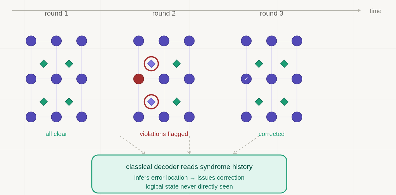
A single round of syndrome measurement gives you a snapshot of which checks are currently flagging violations across the surface. But a single snapshot can be ambiguous. A violation might represent a real error. It might represent a measurement error in the syndrome qubit itself. It might be the tail end of an error chain whose head appeared in a previous round.
This is why syndrome measurement runs continuously, cycle after cycle, throughout the computation. The surface code doesn’t take one picture in effect, it takes a film.
The pattern of violations across time is far more informative than any individual frame. An error on a data qubit appears as a persistent violation. The same check flags in round after round, until the error is corrected. This is really useful because any measurement errors in a syndrome qubit appears as transient violations. That is to say a single measurement error shows up in one round and vanishes in the next, because nothing actually changed on the data qubit being monitored.
The decoding algorithm which sits on the classical software running alongside the quantum hardware reads this three-dimensional record. Two spatial dimensions from the surface, one temporal dimension from the sequence of measurement rounds. It looks for patterns that are consistent with real errors, distinguishes them from measurement noise, and builds the most probable picture of what has actually gone wrong.
Remember this. The error is reconstructed from its history, not from direct observation.
Here is something subtle that becomes important once you look carefully at the syndrome data.
When a chain of errors propagates across the surface a sequence of bit flips on adjacent data qubits, say; the syndrome doesn’t flag the whole chain. It flags only the endpoints.
Think of it this way. Each error in the interior of the chain cancels out its own effect on the local checks. So the violation it would create at one plaquette is compensated by the violation the previous error already created next door. The violations annihilate each other as the chain extends. Only at the two ends, where the chain starts and stops, do unpaired violations remain.
The syndrome data shows you two dots on the surface. The error chain connecting them is invisible. You know something happened between those two points. You don’t know exactly what, or precisely where.
This is both a feature and a challenge. It’s a feature because the decoding problem is now manageable. Instead of trying to locate every individual error across thousands of qubits, you’re trying to pair up the violation endpoints and find the most likely paths connecting them. It’s a challenge because if the error chain is long enough to wrap around the surface and connect its endpoints via a path that crosses the whole lattice, then the correction can fail silently, leaving a logical error behind.
This is precisely what code distance measures. The minimum number of errors required to create such a wraparound chain. Larger surfaces have higher distance, meaning a longer chain is required to cause a logical failure, meaning more errors can be tolerated before the code breaks down.Let’s just pause for a second and reconsider what we’re actually dealing with.
A quantum system is evolving. Noise is acting on it continuously. Errors are occurring at the level of individual physical qubits. And yet the logical information, spread across the surface, encoded in collective correlations remains intact. It remains intact because the errors leave traces in the syndrome data, those traces are read without disturbing the encoded state, and corrections are applied that cancel the errors before they accumulate into something irreversible.
The quantum processor never pauses. The syndrome measurements run in parallel with the computation. The classical decoder works in real time, processing the stream of syndrome data and issuing corrections on a timescale faster than errors build up. The whole system operates as a continuous feedback loop with quantum hardware generating error signals, classical software interpreting them, corrections flowing back.
This is not a theoretical abstraction. It is the operational architecture that any fault-tolerant quantum computer will have to implement. The quantum many-body systems being developed for sensing and simulation face exactly the same landscape. One of continuous noise, continuous monitoring, continuous correction and all running as an integrated process rather than a sequence of discrete steps.
Protecting one logical qubit requires many physical qubits. Running syndrome measurement requires still more. The overhead is real, and it is large. Understanding why that cost exists and whether there are smarter ways to pay it is where we go next.
That’s all for now! If you like my efforts to make quantum science, computing and physical chemistry, more accessible to everyone; please consider recommending this newsletter on your own substack or website. Or share ExoArtDataPulse with a friend or colleague. Every recommend makes the project grow. Thanks for Reading!