

Plotting Entropy
Entropy distribution using matrices and vectors.

Today’s post is inspired by a paper I came across, which is ‘seminal’ for the study of entropy, though I confess I didn’t know that when I came across it. I often go browsing just to see what’s out there and this one is a nugget and a half1.
The paper is Jaynes (1957) , “Information Theory and Statistical Mechanics.” In it, the author argues that statistical mechanics should be understood not as a physical theory grounded in mechanics, but as a form of statistical inference. The paper is a landmark in the foundations of statistical physics.
Jaynes’ central methodological move is a reinterpretation of entropy. Rather than treating entropy as a physical quantity to be derived from microscopic dynamics, he takes it as his starting point by following Shannon’s information-theoretic definition2 and builds statistical mechanics on top of it.
The core procedure is the maximum-entropy principle. When making inferences from incomplete information, one should choose the probability distribution that maximises entropy subject to whatever constraints are known.
Now, let’s step back for a moment and consider what we understand by ‘Entropy’.
You’ve probably heard entropy described as “disorder,” “chaos,” or the universe’s tendency to cool down or even fall apart. However, if entropy were just a metaphor, we couldn’t use it to predict how efficiently an engine converts heat into work, design materials that conduct electricity in exotic ways, or build quantum devices that exploit the rules of probability at the subatomic level.
Specifically, entropy measures how energy is distributed among the possible states of a system not whether the system looks tidy or chaotic.
What counts as a “state”? That depends on the system. For a gas, a state might be a particular arrangement of positions and velocities for every molecule. For a quantum dot, it might be an electron occupying a specific energy level. For a simple coin flip, it might just be heads or tails.
The key insight is that the more states a system could plausibly be in, the higher its entropy.
A system confined to one possible state has very low entropy. A system that could be in any of a trillion (or more) equally likely arrangements has very high entropy3. Entropy, then, is fundamentally about counting and weighing possibilities. hence the power and might of Jayne’s statistical approach.
Think about it. Suppose you have a system with two possible energy states. We can describe it with two numbers, i.e. the probability of being in state 1, and the probability of being in state 2. Simple enough. Now suppose we have four states. We have four numbers. Still manageable.
Now suppose we have a hundred or more states, each of which can transition to any of the others with some probability, and those probabilities depend on temperature, and the energy levels themselves shift when you apply a magnetic field.
At this point, we need a bigger boat. Something that can store all the relevant values at once and represent the relationships between states, not just the states themselves. Furthermore, it needs to scale to large systems without becoming unmanageable and support the kinds of calculations physicists and engineers actually need to do.
This is where matrices come to the fore i.e. grids of numbers, manipulated according to certain rules. But the formal definition can obscure what they are actually for, so think of it this way.
A matrix is a compact way to represent relationships between states.
Consider a physical system with several energy levels. Some transitions between levels are allowed and others are forbidden. Some transitions are highly probable; others are rare. The matrix encoding this system has an entry for every pair of states, thus encoding the strength, probability, or rate of the connection between them.
Think of it as a map of interactions. Every row corresponds to one state. Every column corresponds to another. The number at row i, column j tells you something about the relationship between state i and state j. Perhaps the probability of transitioning from j to i, or the energy coupling between them.
This is why matrices appear everywhere in physics: not because physicists love abstraction, but because many physical questions are fundamentally about how states relate to each other.
Let’s consider energy states as vectors for a minute and how we might represent the current condition of a system? If a system has, say, five energy levels, its current condition might be described by a set of probabilities, one for each level. Maybe there’s a 40% chance of being in level 1, a 30% chance of being in level 2, and so on. Or perhaps the system is definitely in level 3, and the probabilities of all other levels are zero.
This list of values, or ‘weights’, one entry per state, is naturally written as a column vector. Each entry corresponds to one possible state, and the value of that entry tells you how much of the system’s probability (or population, or quantum amplitude) sits in that state.
The vector is not a location in physical space. It is a location in state space. That is, a mathematical space where each dimension corresponds to one possible configuration of the system. This is a subtle but important distinction. We are not asking where the system is geographically; we are asking what it is doing, across all the possibilities open to it.
If we consider how matrices act on vectors we can start to draw the pieces together. For instance, a matrix, applied to a vector, produces a new vector. In the language of state spaces, this means that given the system’s current distribution over states, the matrix tells you what the distribution looks like after some process has acted on it. To be a bit more specific, it works like this;
i. The vector represents the system’s current condition or as we saw earlier, its distribution across states.
ii. The matrix represents the system’s rules in terms of how states evolve, interact, or exchange population.
iii. So applying the rules to the state as it stands, that is, applying the matrix to the vector gives us the system’s condition after one step of evolution!
Apply the matrix again, and we get the condition after a second step. Repeat this many times, and we can trace the full evolution of the system from any starting point to its eventual equilibrium. You can immediately see how we might use this approach to model, or simulate lots of systems4.
Truth be told, this single idea of matrices acting on vectors, repeatedly sits at the heart of a remarkable range of physical theories. It underpins Markov models of random processes. It describes how quantum states evolve over time. It explains how a hot material gradually reaches equilibrium with its surroundings, transferring energy until the distribution of occupied states reaches a stable form. The mathematical approach is the same in all of these cases, even if the physical interpretation differs.
How, then do we go about plotting entropy, which is where we started?
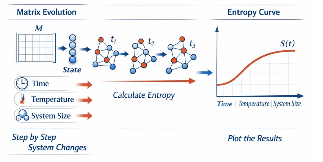
Once we have a matrix model of a system and a vector describing its current state, we can compute entropy as a derived quantity i.e. a number that summarises how spread out the state distribution is. The more evenly probability is distributed across states, the higher the entropy. The more it is concentrated in a few states (or just one), the lower it is.
When we evolve the system step by step using matrix–vector dynamics, whether advancing time, adjusting temperature, or increasing the number of interacting components, we can calculate the entropy at each stage. Plotting those values against time, temperature, or system size produces the smooth, reliable curves familiar from thermodynamics textbooks.
To be clear, in quantum mechanics, the state of a system is still described by a vector. But the entries of that vector are complex numbers called amplitudes, and what we measure are probabilities derived from those amplitudes. Observables i.e. things like energy, momentum, and position are represented by matrices. Measuring an observable collapses the state vector in a specific mathematical way.
Entropy, in the quantum setting, becomes ‘Von Neumann entropy’5 which generalises the classical ideas described here. The language of matrices and vectors remains essential, but the interpretation deepens.
That’s all for now! If you like my efforts to make quantum science, computing and physical chemistry, more accessible to everyone; please consider recommending this newsletter on your own substack or website. Or share ExoArtDataPulse with a friend or colleague. Every recommend makes the project grow. Thanks for Reading!
Edwin T. Jaynes — Information Theory and Statistical Mechanics, (1957) available free to download at https://files.batistalab.com/teaching/attachments/chem584/Jaynes.pdf
Claude Shannon, working at Bell Labs, published A Mathematical Theory of Communication in 1948. His goal was essentially an engineering one. He asked, how do you quantify the information content of a message, and how efficiently can you transmit it down a channel? In solving this, he arrived at a definition of uncertainty or information that turned out to have profound implications far beyond telecommunications.
Shannon proved that these three seemingly modest conditions are enough to uniquely determine the form of the measure, up to a constant scaling factor. The only function satisfying all three is:
H = -Σ(p(x) * log₂(p(x)))
Where:
H is the Shannon entropy
p(x) is the probability of event x occurring
Σ represents the sum over all possible events
This is Shannon entropy, and it measures the ‘average uncertainty’ in a probability distribution. The formula is quoted from the online calculator for Shannon entropy at https://ctrlcalculator.com/statistics/shannon-entropy-calculator/ by Garth C. Clifford.
Take the universe for instance. To say ‘the universe tends to entropy’ does not mean it tends to chaos and collapse. At best it might infer that the universe tends to cool down which again is less than the apocalyptic doom sayers would have us believe. Personally, I would have thought that the universe has a tendency to cool down was blindly obvious but perhaps that’s just me. Even then, you could reasonably argue that ‘cool down’, just means a uniform heat all round. There’s a post of its own on this now I’ve started pulling on the thread.
You can also see how you would structure the research effort. Effort would need to go into describing the system and its components, and effort would need to go into understanding how the system in question evolves, or degrades. From all that, the rest spins out. i.e. the model simulation and information processing stack, reporting requirements, conference attendances, manpower requirements, supervisory approach, peer reviewed papers and so on.
Von Neumann entropy captures two distinct sources of uncertainty in a quantum system. The first is ordinary classical ignorance i.e. you might not know which state the system was prepared in. The second is something more fundamental: even if you know everything quantum mechanics allows you to know about a system, it may still be entangled with something else, making its own state genuinely indefinite. Von Neumann entropy measures both together. Much more on this in the second post of April 2026, just before Easter upcoming.